API documentation

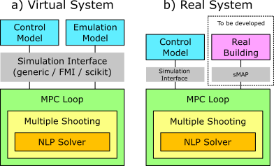
There are two optimization classes to interact with (MPCEmulation and MShoot) and three simulation interfaces (SimModel, SimFMU, SimScikit).

The class MPCEmulation allows to run a virtual MPC experiment, using chosen emulator and control models. The emulator model is a mock-up of a real building. The control model is used by the optimization solver to find the optimal control trajectory. Each optimization horizon in the MPC loop is automatically optimized using MShoot.

Both, the emulator and control models have to be interfaced via one of the available interfaced classes. SimModel is the generic interface or wrapper, which can be used to wrap any Python model. SimFMU is the interface to Functional Mock-up Units. SimScikit is the interface to scikit-learn models.

The class MShoot allows to run a single optimal control problem (for a single time period), using the multiple shooting method. Therefore, only one model is needed, equivalent to the control model used in MPCEmulation. This class is automatically used in the MPC loop in MPCEmulation.

How to set up MPCEmulation

1. Instantiate the emulator model using SimModel, SimFMU, or SimScikit:

model_emu = mshoot.SimFMU(
    fmupath,
    outputs=['qout', 'Tr'],
    states=['heatCapacitor.T'],
    parameters={'C': 1e6, 'R': 0.01},
    verbose=False)

2. Instantiate the control model using SimModel, SimFMU, or SimScikit

model_ctr = mshoot.SimFMU(
    fmupath,
    outputs=['qout', 'Tr'],
    states=['heatCapacitor.T'],
    parameters={'C': 1e6, 'R': 0.01},
    verbose=False)

3. Define the cost function:

# This function is passed to MPCEmulation
def cfun(xdf, ydf):
    """
    :param ydf: DataFrame, model states
    :param ydf: DataFrame, model outputs
    :return: float
    """
    qout = ydf['qout']
    c = np.sum(qout ** 2) / qout.size
    return c

4. Define control and emulator model inputs. The inputs have to be stored in data frames with an equidistant index (named time) in seconds. The emulator and input data frames have to be aligned with respect to each other (using same index). The time step used in index is also used as the simulation time step, and is used as the base unit for defining the optimization horizon length. E.g. horizon = 3 means that the optimization horizon is three time steps long.

# Inputs
tstep = 3600.  # s
tend = 3600. * 48
t = np.arange(0., tend + 1, tstep)
q = np.full(t.size, 0.)
Tout  = np.sin(t / 86400. * 2. * np.pi) + 273.15

inp = pd.DataFrame(
    index=pd.Index(t, name='time'),
    columns=['q', 'Tout'],
    data=np.vstack((q, Tout)).T
)

5. Define state bounds (scalars for constant or vectors for time-dependent):

h = t / 3600.  # auxiliary variable (time in hours)

# Lower constraint (time-dependent example)
Tlo = np.where((h >= 8) & (h <= 17), 21. + 273.15, 21. + 273.15)

# Upper constraint (constant example)
Thi = 297.15

6. Instantiate MPCEmulation:

mpc = mshoot.MPCEmulation(model_emu, cfun)

7. Optimize:

u, xctr, xemu, yemu, u_hist = mpc.optimize(
    model=model_ctr,        # control model instance
    inp_ctr=inp,            # control model inputs
    inp_emu=inp,            # emulator model inputs
    free=['q'],             # control inputs
    ubounds=[(0., 5000.)],  # control input bounds
    xbounds=[(Tlo, Thi)],   # state constraints
    x0=[294.15],            # initial state
    maxiter=30,             # max. number of NLP iterations
    ynominal=[5000., 20.],  # nominal control model outputs
    step=1,                 # distance between control horizons
    horizon=3               # control horizon length
)

How to set up MShoot

1. Instantiate the model using SimModel, SimFMU, or SimScikit:

model = mshoot.SimFMU(
    fmupath,
    outputs=['qout', 'Tr'],
    states=['heatCapacitor.T'],
    parameters={'C': 1e6, 'R': 0.01},
    verbose=False)

2. Define the cost function:

def cfun(xdf, ydf):
    """
    :param ydf: DataFrame, model states
    :param ydf: DataFrame, model outputs
    :return: float
    """
    qout = ydf['qout'].values
    c = np.sum(qout ** 2) / qout.size
    return c

3. Define the inputs:

t = np.arange(0, 3600 * 10, 3600)
inp = pd.DataFrame(index=pd.Index(t, name='time'), columns=['q', 'Tout'])
inp['q'] = np.full(t.size, 0.)
inp['Tout'] = np.full(t.size, 273.15)

4. Define the input and state bounds (scalars for constant or vectors for time-dependent):

ubounds = [(0., 4000.)]
xbounds = [(293.15, 296.15)]

5. Instantate MShoot:

ms = mshoot.MShoot(cfun=cfun)

6. Optimize:

udf, xdf = mpc.optimize(
    model=get_model(),
    inp=inp,
    free=['q'],
    ubounds=ubounds,
    xbounds=xbounds,
    x0=x0,
    uguess=None,
    ynominal=[4000, 295.],
    join=1,
    maxiter=30
)

Docstrings

• MPCEmulation
• MShoot
• Simulation interfaces